
Budker group Berkeley Tutorials
Danila Barskiy Tutorials
Six-wire transmission line
by Manas Pandey
Dipole-Dipole Interactions Explained
by Dr. Danila Barskiy
Interactions between spins are fundamental for understanding magnetic resonance. One of the most important ones is the magnetic dipole-dipole interaction. Spins act as tiny magnets, thus, they can interact with each other directly through space, pretty much the same way as classical magnetic dipoles (Figure 1). In NMR, dipole-dipole interactions very often determine lineshapes of solid-state samples and relaxation rates of nuclei in the liquid state.

Figure 1. Nuclear spin 1 produces the magnetic field that is sensed by a spin 2. Similarly, nuclear spin 2 produces the magnetic field that is sensed by a spin 1.
In many NMR textbooks, you can find the following expression for dipole-dipole (DD) Hamiltonian between two spins 1 and 2:
$\hat{{H}}_{\rm DD} = d_{12} \left( 3 \hat{I}_{1z} \hat{I}_{2z} – \hat{\mathbf{I}}_1 \cdot \hat{\mathbf{I}}_2 \right) ,$
where $ d_{12} = – \displaystyle\frac{\mu_0}{4 \pi} \displaystyle\frac{\gamma_1 \gamma_2 \hbar}{r^3} \frac{\left( 3 \cos^2{\theta} – 1 \right)}{2} $, $ \gamma_1 $ and $ \gamma_2 $ are gyromagnetic ratios of the spins, $ r$ is the distance between them. Meaning of the angle $ \theta $ can be seen from the Figure 2. But how was this expression derived?
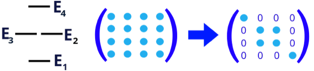
Figure 2. Two nuclear spins, 1 and 2, are separated by the distance r. $ \theta $ is defined as an angle between z-direction of the coordinate system and the vector connecting the two spins. If there is an external magnetic field B0, it is usually defined along the z-axis.
In physics, I rarely struggled with imagining abstract things and concepts, but rather, I was often lazy to do math thoroughly and derive equations from the beginning to the end. That’s why I decided to write here a full derivation, from the beginning to the end, for the Hamiltonian of interacting nuclear spins. We will start from a classical expression of the magnetic field produced by the dipole and finish by the analysis of a truncated dipole-dipole Hamiltonian. Usually, you don’t see such a full derivation in textbooks. Maybe, this is because textbooks have limited space… Luckily, here we do not have such limitations, thus, we can have some fun here! Let’s go then! 🙂
Classical equation describing the magnetic field $ \vec{\boldsymbol{B}}_{\rm dip} (\vec{\boldsymbol{r}}) $ produced by a magnetic dipole moment $ \vec{\boldsymbol{\mu}}$ is
$ \vec{\boldsymbol{B}}_{\rm dip} (\vec{\boldsymbol{r}}) = \displaystyle\frac{\mu_0}{4 \pi r^3} \left( 3 \left( \vec{\boldsymbol{\mu}} \cdot \hat{\boldsymbol{r}} \right) \hat{\boldsymbol{r}} – \vec{\boldsymbol{\mu}} \right) , $
where $ \hat{\boldsymbol{r}} = \displaystyle\frac{\vec{\boldsymbol{r}}}{|\vec{\boldsymbol{r}}|}$ is a unit vector. It is easy to show that $ \left( \vec{\boldsymbol{\mu}} \cdot \vec{\boldsymbol{r}} \right) \vec{\boldsymbol{r}} = \left( \vec{\boldsymbol{r}} \cdot \vec{\boldsymbol{r}}^{\: \intercal} \right) \vec{\boldsymbol{\mu}} $.
Indeed,
$ \left( \vec{\boldsymbol{\mu}} \cdot \vec{\boldsymbol{r}} \right) \vec{\boldsymbol{r}} = \left( \mu_x r_x + \mu_y r_y + \mu_z r_z \right) \cdot
\begin{pmatrix}
r_x \\
r_y \\
r_z
\end{pmatrix}
=$
$\begin{pmatrix}
\mu_{x} r_{x} r_{x} + \mu_{y} r_{y} r_{x} + \mu_{z} r_{z} r_{x} \\
\mu_{x} r_{x} r_{y} + \mu_{y} r_{y} r_{y} + \mu_{z} r_{z} r_{y} \\
\mu_{x} r_{x} r_{z} + \mu_{y} r_{y} r_{z} + \mu_{z} r_{z} r_{z}
\end{pmatrix} $
which is the same as
$
\left( \vec{\boldsymbol{r}} \cdot \vec{\boldsymbol{r}}^{\: \intercal} \right) \vec{\boldsymbol{\mu}}
=$ $
\begin{pmatrix}
r_{x} r_{x} & r_{x} r_{y} & r_{x} r_{z} \\
r_{y} r_{x} & r_{y} r_{y} & r_{y} r_{z} \\
r_{z} r_{x} & r_{z} r_{y} & r_{z} r_{z}
\end{pmatrix} \cdot
\begin{pmatrix}
\mu_x \\
\mu_y \\
\mu_z
\end{pmatrix} = $ $
\begin{pmatrix}
r_{x} r_{x} \mu_{x} + r_{x} r_{y} \mu_{y} + r_{x} r_{z} \mu_{z} \\
r_{y} r_{x} \mu_{x} + r_{y} r_{y} \mu_{y} + r_{y} r_{z} \mu_{z} \\
r_{z} r_{x} \mu_{x} + r_{z} r_{y} \mu_{y} + r_{z} r_{z} \mu_{z}
\end{pmatrix} .
$
Thus we write the magnetic field produced by a magnetic dipole $ \vec{\boldsymbol{\mu}}_2$ as
$
\vec{\boldsymbol{B}}_{\mu_2} = \displaystyle\frac{\mu_0}{4 \pi r^3} \left( 3 \left( \hat{\boldsymbol{r}} \cdot \hat{\boldsymbol{r}}^{\: \intercal} \right) \vec{\boldsymbol{\mu}}_2 – \vec{\boldsymbol{\mu}}_2 \right) .
$
The energy of a magnetic dipole $ \vec{\boldsymbol{\mu}}_1 $ interacting with the magnetic field $ \vec{\boldsymbol{B}}_{\mu_2}$ produced by a magnetic dipole $ \vec{\boldsymbol{\mu}}_2$ (dipole-dipole interaction) is therefore
$ E_{\rm DD} = – \left( \vec{\boldsymbol{\mu}}_1 \cdot \vec{\boldsymbol{B}}_{\mu_2} \right) = -\displaystyle\frac{\mu_0}{4 \pi r^3} \left( 3 \cdot \vec{\boldsymbol{\mu}}_1 \left( \hat{\boldsymbol{r}} \cdot \hat{\boldsymbol{r}}^{\: \intercal} \right) \vec{\boldsymbol{\mu}}_2 – \left( \vec{\boldsymbol{\mu}}_1 \cdot \vec{\boldsymbol{\mu}}_2 \right) \right) .$
The transition from classical to quantum mechanics is realized by substituting the measurable quantities by corresponding quantum mechanical operators:
$ E_{\rm DD} \rightarrow \hat{H}_{\rm DD} \quad \vec{\boldsymbol{\mu}}_1 \rightarrow \gamma_1 \hbar \hat{\mathbf{I}}_1\quad \vec{\boldsymbol{\mu}}_2 \rightarrow \gamma_2 \hbar \hat{\mathbf{I}}_2$
$ \label{Eq_Hdd}
\hat{H}_{\rm DD} = – \displaystyle\frac{\mu_0}{4 \pi } \displaystyle\frac{\gamma_1 \gamma_1 \hbar}{r^3} \left( 3 \cdot \hat{\mathbf{I}}_1 \left( \hat{\boldsymbol{r}} \cdot \hat{\boldsymbol{r}}^{\: \intercal} \right) \hat{\mathbf{I}}_2 – \left( \hat{\mathbf{I}}_1 \cdot \hat{\mathbf{I}}_2 \right) \right) = b_{12} \hat{\mathbf{I}}_1 \hat{\mathbf{D}} \hat{\mathbf{I}}_2 . $
Here $ b_{12}$ is a factor which depends only on the types of the nuclear spins and the distance between them, and a tensor of dipole-dipole interactions contains information about the mutual orientation of two spins:
$ \hat{\mathbf{D}} = 3 \cdot \left( \hat{\boldsymbol{r}} \cdot \hat{\boldsymbol{r}}^{\: \intercal} \right) – \hat{1} . $
Here $ \hat{1}$ is a unit matrix. Note that we write Hamiltonian $ \hat{H}_{\rm DD}$ in units of [rad/s], that is why one $ \hbar$ is missing. In spherical coordinates:
$ \hat{\boldsymbol{r}} =
\begin{pmatrix}
\sin{\theta} \cos{\phi} \\
\sin{\theta} \sin{\phi} \\
\cos{\theta}
\end{pmatrix} .$
Therefore,
$ \hat{\mathbf{D}} =
\begin{pmatrix}
3 \sin^2{\theta} \cos^2{\phi} – 1 & 3 \sin^2{\theta} \cos{\phi} \sin{\phi} & 3 \sin{\theta} \cos{\theta} \cos{\phi} \\
3 \sin^2{\theta} \cos{\phi} \sin{\phi} & 3 \sin^2{\theta} \sin^2{\phi} – 1 & 3 \sin{\theta} \cos{\theta} \sin{\phi} \\
3 \sin{\theta} \cos{\theta} \cos{\phi} & 3 \sin{\theta} \cos{\theta} \sin{\phi} & 3 \cos^2{\theta} – 1
\end{pmatrix} .$
Looks good, doesn’t it? Now, let’s evaluate the product $ \hat{\mathbf{I}}_1 \hat{\mathbf{D}} \hat{\mathbf{I}}_2$:
$ \hat{\mathbf{I}}_1 \hat{\mathbf{D}} \hat{\mathbf{I}}_2 = $ $
\begin{pmatrix}
\hat{I}_{1x} & \hat{I}_{1y} & \hat{I}_{1z}
\end{pmatrix} \cdot $ $ \cdot
\begin{pmatrix}
3 \sin^2{\theta} \cos^2{\phi} – 1 & 3 \sin^2{\theta} \cos{\phi} \sin{\phi} & 3 \sin{\theta} \cos{\theta} \cos{\phi} \\
3 \sin^2{\theta} \cos{\phi} \sin{\phi} & 3 \sin^2{\theta} \sin^2{\phi} – 1 & 3 \sin{\theta} \cos{\theta} \sin{\phi} \\
3 \sin{\theta} \cos{\theta} \cos{\phi} & 3 \sin{\theta} \cos{\theta} \sin{\phi} & 3 \cos^2{\theta} – 1
\end{pmatrix}
\begin{pmatrix}
\hat{I}_{2x} \\
\hat{I}_{2y} \\
\hat{I}_{2z}
\end{pmatrix} = $
$ \begin{pmatrix}
\hat{I}_{1x} & \hat{I}_{1y} & \hat{I}_{1z}
\end{pmatrix} \cdot $ $
\begin{pmatrix}
\hat{I}_{2x} \left( 3 \sin^2{\theta} \cos^2{\phi} – 1 \right) + \hat{I}_{2y} \left( 3 \sin^2{\theta} \cos{\phi} \sin{\phi} \right) + \hat{I}_{2z} \left( 3 \sin{\theta} \cos{\theta} \cos{\phi} \right) \\
\hat{I}_{2x} \left( 3 \sin^2{\theta} \cos{\phi} \sin{\phi} \right) + \hat{I}_{2y} \left( 3 \sin^2{\theta} \sin^2{\phi} – 1 \right) + \hat{I}_{2z} \left( 3 \sin{\theta} \cos{\theta} \sin{\phi} \right) \\
\hat{I}_{2x} \left( 3 \sin{\theta} \cos{\theta} \cos{\phi} \right) + \hat{I}_{2y} \left( 3 \sin{\theta} \cos{\theta} \sin{\phi} \right) + \hat{I}_{2z} \left( 3 \cos^2{\theta} – 1 \right)
\end{pmatrix} $
$ = \hat{I}_{1x} \hat{I}_{2x}
\left( 3 \sin^2{\theta} \cos^2{\phi} – 1 \right) +
\hat{I}_{1x} \hat{I}_{2y}
\left( 3 \sin^2{\theta} \cos{\phi} \sin{\phi} \right) + $ $ +
\hat{I}_{1x} \hat{I}_{2z}
\left( 3 \sin{\theta} \cos{\theta} \cos{\phi} \right) + \hat{I}_{1y} \hat{I}_{2x}
\left( 3 \sin^2{\theta} \cos{\phi} \sin{\phi} \right) +
\hat{I}_{1y} \hat{I}_{2y}
\left( 3 \sin^2{\theta} \sin^2{\phi} – 1 \right) + $ $ +
\hat{I}_{1y} \hat{I}_{2z}
\left( 3 \sin{\theta} \cos{\theta} \sin{\phi} \right) + + \hat{I}_{1z} \hat{I}_{2x}
\left( 3 \sin{\theta} \cos{\theta} \cos{\phi} \right) +
\hat{I}_{1z} \hat{I}_{2y}
\left( 3 \sin{\theta} \cos{\theta} \sin{\phi} \right) +
\hat{I}_{1z} \hat{I}_{2z}
\left( 3 \cos^2{\theta} – 1 \right) .$
Let’s color terms to make it easier grouping them:
$ \color{red}{\hat{I}_{1x} \hat{I}_{2x}
\left( 3 \sin^2{\theta} \cos^2{\phi} – 1 \right)} + $ $ \color{blue}{\hat{I}_{1x} \hat{I}_{2y}
\left( 3 \sin^2{\theta} \cos{\phi} \sin{\phi} \right)} + $ $ \color{magenta}{\hat{I}_{1x} \hat{I}_{2z}
\left( 3 \sin{\theta} \cos{\theta} \cos{\phi} \right)} + $ $ \color{blue}{\hat{I}_{1y} \hat{I}_{2x}
\left( 3 \sin^2{\theta} \cos{\phi} \sin{\phi} \right)} + $ $ \color{red}{\hat{I}_{1y} \hat{I}_{2y} \left( 3 \sin^2{\theta} \sin^2{\phi} – 1 \right)} + $ $ \color{magenta}{\hat{I}_{1y} \hat{I}_{2z} \left( 3 \sin{\theta} \cos{\theta} \sin{\phi} \right)} + $ $ \color{magenta}{\hat{I}_{1z} \hat{I}_{2x}
\left( 3 \sin{\theta} \cos{\theta} \cos{\phi} \right)} +
\color{magenta}{\hat{I}_{1z} \hat{I}_{2y}
\left( 3 \sin{\theta} \cos{\theta} \sin{\phi} \right)} + $ $ \hat{I}_{1z} \hat{I}_{2z} \left( 3 \cos^2{\theta} – 1 \right) .$
Grouping the red terms gives
$ \color{red}{\left( \hat{I}_{1x} \hat{I}_{2x} \cos^2{\phi} + \hat{I}_{1y} \hat{I}_{2y} \sin^2{\phi} \right) 3 \sin^2{\theta}
– \left( \hat{I}_{1x} \hat{I}_{2x} + \hat{I}_{1y} \hat{I}_{2y} \right)} .$
Let’s not forget about intrinsic connections of spin angular momentum with raising and lowering operators:
$ \hat{I}_{1x} \hat{I}_{2x} =
\displaystyle\frac{\left( \hat{I}_{1+} + \hat{I}_{1-} \right)}{2}\displaystyle\frac{\left( \hat{I}_{2+} + \hat{I}_{2-} \right)}{2} =
\displaystyle\frac{1}{4} \left( \hat{I}_{1+} \hat{I}_{2+} + \hat{I}_{1+} \hat{I}_{2-} + \hat{I}_{1-} \hat{I}_{2+} + \hat{I}_{1-} \hat{I}_{2-} \right) $
$ \hat{I}_{1y} \hat{I}_{2y} =
\displaystyle\frac{\left( \hat{I}_{1+} – \hat{I}_{1-} \right)}{2 i}\displaystyle\frac{\left( \hat{I}_{2+} – \hat{I}_{2-} \right)}{2 i} =
-\displaystyle\frac{1}{4} \left( \hat{I}_{1+} \hat{I}_{2+} – \hat{I}_{1+} \hat{I}_{2-} – \hat{I}_{1-} \hat{I}_{2+} + \hat{I}_{1-} \hat{I}_{2-} \right) .$
Therefore, grouping the red terms gives
$ \color{red}{\left( \hat{I}_{1x} \hat{I}_{2x} \cos^2{\phi} + \hat{I}_{1y} \hat{I}_{2y} \sin^2{\phi} \right) 3 \sin^2{\theta} – \left( \hat{I}_{1x} \hat{I}_{2x} + \hat{I}_{1y} \hat{I}_{2y} \right) =} $ $\color{red}{= \left( \hat{I}_{1+} \hat{I}_{2-} + \hat{I}_{1-} \hat{I}_{2+} \right) \frac{3}{4} \sin^2{\theta} + \left( \hat{I}_{1+} \hat{I}_{2+} + \hat{I}_{1-} \hat{I}_{2-} \right) \frac{3}{4} \sin^2{\theta} \cdot \left( \cos{ 2 \phi} \right)} $ $ \color{red}{- \frac{1}{2} \left( \hat{I}_{1+} \hat{I}_{2-} + \hat{I}_{1-} \hat{I}_{2+} \right) = \left( \hat{I}_{1+} \hat{I}_{2-} + \hat{I}_{1-} \hat{I}_{2+} \right) \frac{1}{4} \left(1 – 3 \cos^2{\theta} \right)} $ $ \color{red}{- \left( \hat{I}_{1+} \hat{I}_{2+} + \hat{I}_{1-} \hat{I}_{2-} \right) \frac{3}{4} \sin^2{\theta} \cdot \left( \cos{ 2 \phi} \right)} .$
Grouping the blue terms gives
$ \color{blue}{\left( \hat{I}_{1x} \hat{I}_{2y} + \hat{I}_{1y} \hat{I}_{2x} \right) 3 \sin^2{\theta} \cos{\phi} \sin{\phi} = \left( \hat{I}_{1+} \hat{I}_{2+} – \hat{I}_{1-} \hat{I}_{2-} \right)\displaystyle\frac{3}{4} \sin^2{\theta} \cdot \left( – i \sin{2 \phi} \right)} ,$
where we took into consideration that
$ \hat{I}_{1x} \hat{I}_{2y} =\displaystyle\frac{\left( \hat{I}_{1+} + \hat{I}_{1-} \right)}{2} \frac{\left( \hat{I}_{2+} – \hat{I}_{2-} \right)}{2 i} =
\frac{1}{4 i} \left( \hat{I}_{1+} \hat{I}_{2+} – \hat{I}_{1+} \hat{I}_{2-} + \hat{I}_{1-} \hat{I}_{2+} – \hat{I}_{1-} \hat{I}_{2-} \right) $
$ \hat{I}_{1y} \hat{I}_{2x} = \displaystyle\frac{\left( \hat{I}_{1+} – \hat{I}_{1-} \right)}{2 i} \frac{\left( \hat{I}_{2+} + \hat{I}_{2-} \right)}{2} =
\frac{1}{4 i} \left( \hat{I}_{1+} \hat{I}_{2+} + \hat{I}_{1+} \hat{I}_{2-} – \hat{I}_{1-} \hat{I}_{2+} – \hat{I}_{1-} \hat{I}_{2-} \right) .$
Red and blue terms can be combined nicely to form
$ \left( \hat{I}_{1+} \hat{I}_{2-} + \hat{I}_{1-} \hat{I}_{2+} \right) \displaystyle\frac{1}{4} \left(1 – 3 \cos^2{\theta} \right) + \hat{I}_{1+} \hat{I}_{2+} \left( \frac{3}{4} \sin^2{\theta} \cdot e^{- 2 i \phi} \right) + \hat{I}_{1-} \hat{I}_{2-} \left( \frac{3}{4} \sin^2{\theta} \cdot e^{+ 2 i \phi} \right) .$
Now let’s focus on purple terms:
$ \color{magenta}{\left( \hat{I}_{1x} \hat{I}_{2z} + \hat{I}_{1z} \hat{I}_{2x} \right) \left( \hat{I}_{1x} \hat{I}_{2z} + \hat{I}_{1z} \hat{I}_{2x} \right) \left( 3 \sin{\theta} \cos{\theta} \cos{\phi} \right)} $ $ \color{magenta}{+ \left( \hat{I}_{1y} \hat{I}_{2z} + \hat{I}_{1z} \hat{I}_{2y} \right) \left( 3 \sin{\theta} \cos{\theta} \sin{\phi} \right) =} $ $ \color{magenta}{= \left( \left( \hat{I}_{1+} \hat{I}_{2z} + \hat{I}_{1-} \hat{I}_{2z} + \hat{I}_{1z} \hat{I}_{2+} + \hat{I}_{1z}\hat{I}_{2-} \right) \cos{\phi} \right) \displaystyle\frac{3}{4} \sin{2 \theta}} $ $ \color{magenta}{+ \left( \left( -i \hat{I}_{1+} \hat{I}_{2z} + i \hat{I}_{1-} \hat{I}_{2z} -i \hat{I}_{1z} \hat{I}_{2+} + i \hat{I}_{1z} \hat{I}_{2-} \right) \sin{\phi} \right) \frac{3}{4} \sin{2 \theta} =} $ $ \color{magenta}{= \left( \hat{I}_{1+} \hat{I}_{2z} + \hat{I}_{1z} \hat{I}_{2+} \right) \left( \frac{3}{4} \sin{2 \theta} \right) e^{-i \phi} + \left( \hat{I}_{1-} \hat{I}_{2z} + \hat{I}_{1z} \hat{I}_{2-} \right) \left( \frac{3}{4} \sin{2 \theta} \right) e^{+i \phi}} .$
Overall, we have split our dipolar Hamiltonian into six terms, the so-called “Dipolar Alphabet”:
$ \hat{\mathbf{I}}_1 \hat{\mathbf{D}} \hat{\mathbf{I}}_2 = \hat{A} + \hat{B} + \hat{C} + \hat{D} + \hat{E} + \hat{F} ,$
where
$ \hat{A} \quad = \quad \hat{I}_{1z} \hat{I}_{2z} \left( 3 \cos^2{\theta} – 1 \right) $
$ \hat{B} \quad = \quad \left( \hat{I}_{1+} \hat{I}_{2-} + \hat{I}_{1-} \hat{I}_{2+} \right) \cdot \displaystyle\frac{\left(1 – 3 \cos^2{\theta} \right)}{4} $
$ \hat{C} \quad = \quad \left( \hat{I}_{1+} \hat{I}_{2z} + \hat{I}_{1z} \hat{I}_{2+} \right) \left( \displaystyle\frac{3}{4} \sin{2 \theta} \right) e^{-i \phi} $
$ \hat{D} \quad = \quad \left( \hat{I}_{1-} \hat{I}_{2z} + \hat{I}_{1z} \hat{I}_{2-} \right) \left( \displaystyle\frac{3}{4} \sin{2 \theta} \right) e^{+i \phi} $
$ \hat{E} \quad = \quad \hat{I}_{1+} \hat{I}_{2+} \left( \displaystyle\frac{3}{4} \sin^2{\theta} \right) e^{- 2 i \phi} $
$ \hat{F} \quad = \quad \hat{I}_{1-} \hat{I}_{2-} \left( \displaystyle\frac{3}{4} \sin^2{\theta} \right) e^{+ 2 i \phi} .$
To summarize, the Hamiltonian of two interacting spins is a $ 4 \times 4 $ matrix composed of 6 operators. Each of the letters of the dipolar alphabet corresponds to certain matrix elements in the final Hamiltonian (Figure 3).
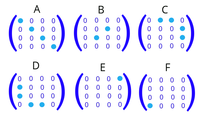
Figure 3. If written in Zeeman basis (αα, αβ, βα and ββ), dipole-dipole Hamiltonian can be split into the following six terms of the “Dipolar Alphabet”.
Without an externally imposed direction in space (for example, in the case of two equivalent spins in zero magnetic field), all of the terms of the dipole-dipole Hamiltonian need to be used for calculating an NMR spectrum. This is because all orientations in space are equivalent. However, in the presence of the external high magnetic field, the Hamiltonian can be simplified via the use of so-called “secular approximation”.
The secular approximation concerns the case where the Hamiltonian is the sum of two terms:
$ \hat{H} = \hat{A} + \hat{B} ,$
where $ \displaystyle\hat{A} $ is a “large” operator and $ \hat{B} $ is a “small” operator. In our case, $ \hat{A} $ can be an operator describing the interaction with the magnetic field (Zeeman Hamiltonian) and $ \hat{B} $ is DD Hamiltonian. Eigenstates of the Zeeman Hamiltonian are familiar αα, αβ, βα, ββ. Generally, $ \hat{B} $ does not commute with $ \hat{A} $, therefore, if written in the eigenbasis of $ \hat{A}$, it has finite elements everywhere.
The secular approximation for $ \hat{B} $ means that we leave only the blocks that correspond to the eigenvalue structure of the operator $ \hat{A}$ (Figure 4) and disregard all other elements.
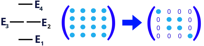
Figure 4. Energy level structure of the Zeeman Hamiltonian: lowest energy level (E1) corresponds to the state αα, energy levels E2 and E3 correspond to the states αβ and βα. The highest energy level (E4) corresponds to the nuclear spin state ββ. The essence of secular approximation is to make the to-be-simplified Hamiltonian match the eigenvalue structure of the main Hamiltonian. One can see from Figure 3 that the first two terms of the DD Hamiltonian will match the structure of the Zeeman Hamiltonian.
In general, we can omit a matrix element $ b_{nm} $ that is much smaller than
$ |b_{mn}| \ll |E_m – E_n| .$
For homonuclear case (e.g., two interacting protons), this means that only the first two terms of the dipolar Alphabet will survive:
$ \hat{\mathbf{I}}_1 \hat{\mathbf{D}} \hat{\mathbf{I}}_2 = \hat{A} + \hat{B} = $
$ = \hat{I}_{1z} \hat{I}_{2z} \left( 3 \cos^2{\theta} – 1 \right) + \left( \hat{I}_{1+} \hat{I}_{2-} + \hat{I}_{1-} \hat{I}_{2+} \right) \cdot \displaystyle\frac{\left(1 – 3 \cos^2{\theta} \right)}{4} = $
$ = \hat{I}_{1z} \hat{I}_{2z} \left( 3 \cos^2{\theta} – 1 \right) – \left( \hat{I}_{1x} \hat{I}_{2x} + \hat{I}_{2y} \hat{I}_{2y} \right) \cdot \displaystyle\frac{\left(3 \cos^2{\theta} – 1\right)}{2} = $
$ = \displaystyle\frac{\left( 3 \cos^2{\theta} – 1\right)}{2} \cdot \left( 2 \hat{I}_{1z} \hat{I}_{2z} + \hat{I}_{1z} \hat{I}_{2z} – \hat{I}_{1z} \hat{I}_{2z} – \left( \hat{I}_{1x} \hat{I}_{2x} + \hat{I}_{2y} \hat{I}_{2y} \right) \right) =$
$ = \displaystyle\frac{\left(3 \cos^2{\theta} – 1\right)}{2} \cdot \left( 3 \hat{I}_{1z} \hat{I}_{2z} – \hat{\mathbf{I}}_1 \cdot \hat{\mathbf{I}}_2 \right) .$
Overall, this is how you go from the classical description of the magnetic field of the dipole to the truncated form of the Hamiltonian in the high magnetic field. In the next post I will show how this Hamiltonian leads to the characteristic lineshape of the NMR line for solids.